Data-Efficient Model Validation
Fait Poms*, Vishnu Sarukkai*, Ravi Teja Mullapudi, Nimit Sohoni, Bill Mark, Deva Ramanan, and Kayvon Fatahalian
In recent years, the machine learning community has made significant progress towards reducing the amount of labeled training data required to build effective models. In the computer vision community, semi-supervised techniques such as SwAV make it possible to train competitive models with labels for less than 5% of the ImageNet train dataset.
However, when constructing a model from scratch, both training and validation require labeled data. Having reduced labeling budgets for training, validation dominates overall labeling costs. Therefore, reducing validation labeling costs is essential to reducing overall labeling costs for model creation.
Problem Setup
In ICCV 2021, our paper focuses on sample-efficient model validation for binary classifiers for rare categories. These classifiers are valuable across a variety of real-world scenarios, and rare categories pose a particularly difficult problem for validation because of how hard it is to find the positive instances in the dataset.
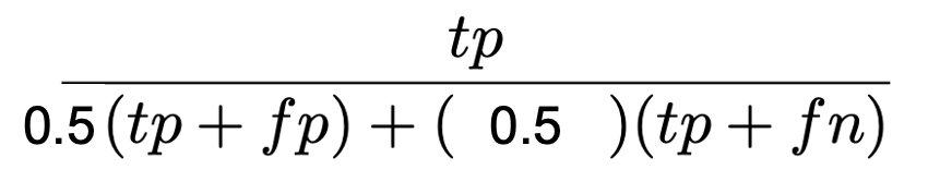
We aim to estimate the F-Score of our binary classifiers. F-Scores are a generalized family of metrics that depend on true positive (tp), false positive (fp), and false negative (fn) counts. The equation is parameterized by alpha:
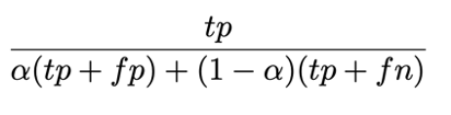
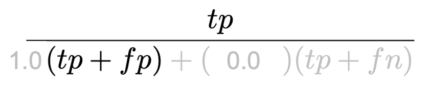
Setting alpha to different values yields several common validation metrics. Setting alpha to 1, we can compute precision:
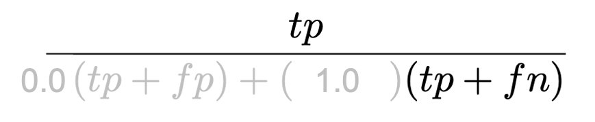
Setting alpha to 0, we can compute recall:
Setting alpha to 0.5, we can compute F1:
Typically, in the computer vision community, we validate by calculating the value of the F-Score given a large, fully-labeled validation set. Instead, our work views the computation of F-Scores as a statistical estimation procedure where the goal is to estimate the F-Score that would have been computed if we had access to a huge, labeled dataset.
Method
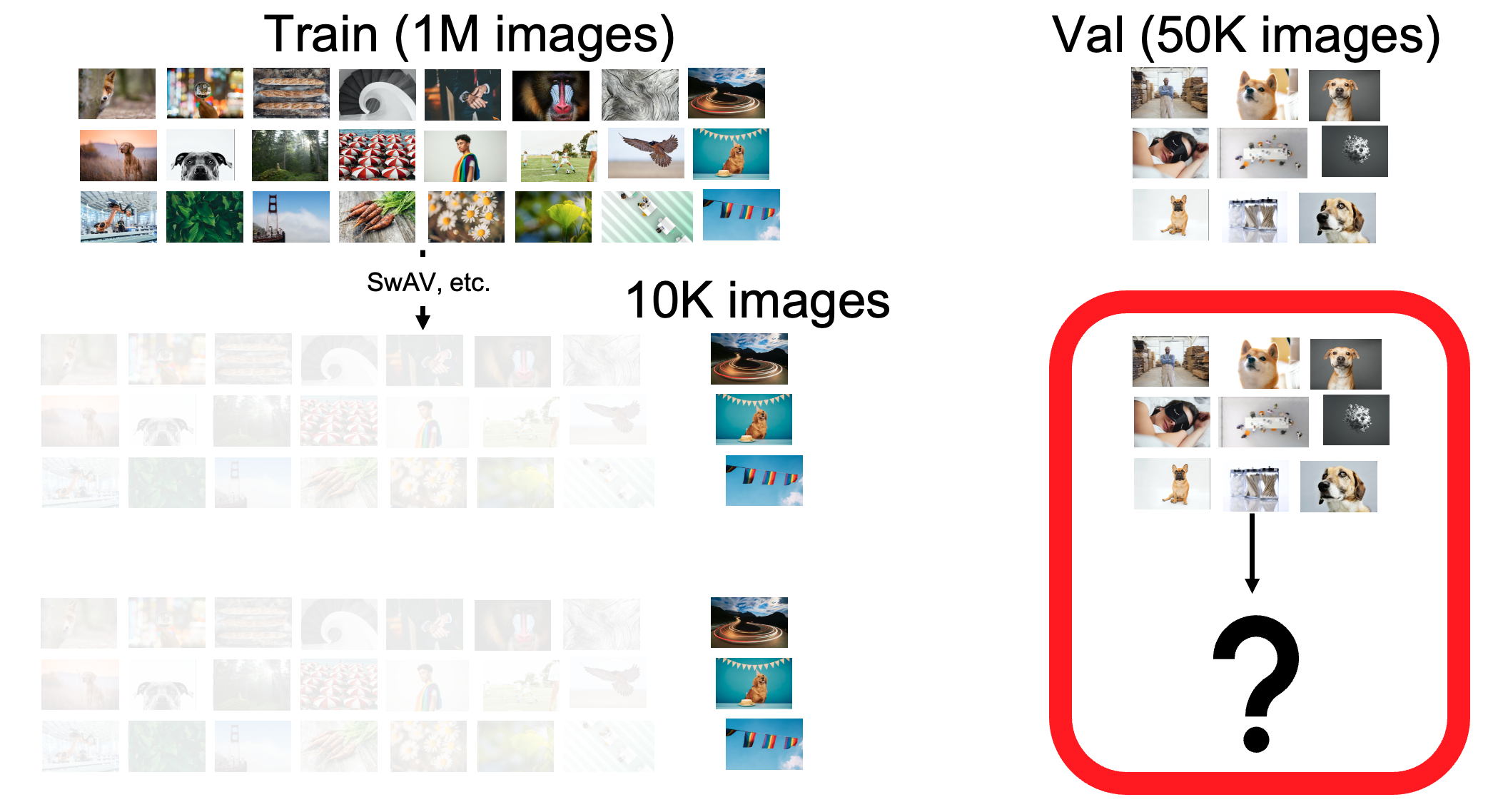
The most straightforward approach to estimating F-Scores is to select a random subset of images, label them, and then estimate the F-Score based on this random subset. Unfortunately, while this procedure may be “correct” in expectation, the generate estimates have high variance. To get a sense of how extreme this might be in practice, suppose a dog breed is present in one-thousandth of images in ImageNet. When selecting 50 images at random, 95% of the time we wouldn’t even find a single dog.
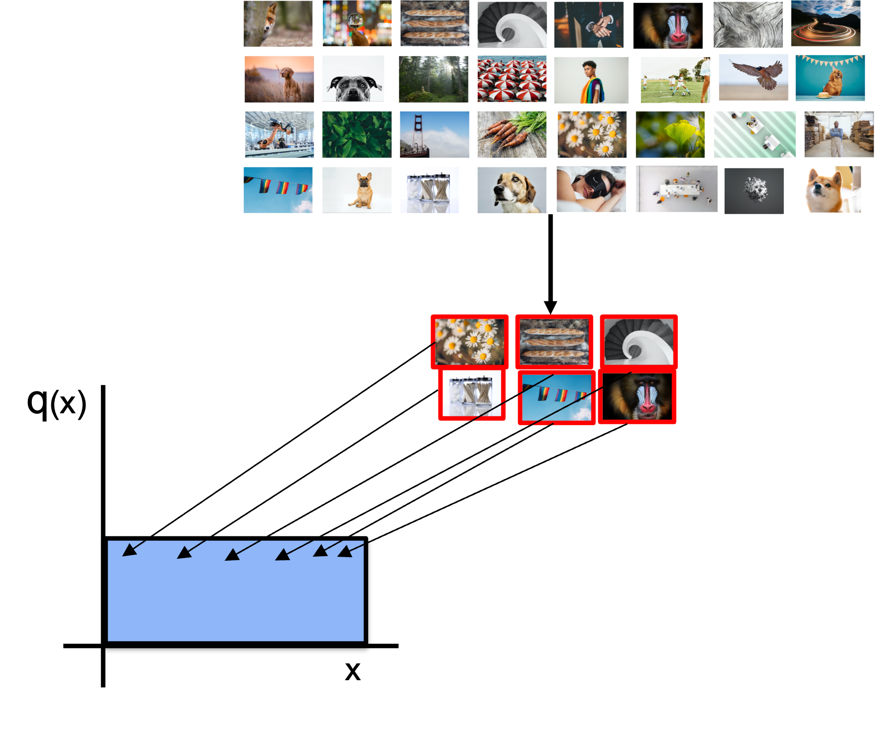
Instead of sampling uniformly, it is common in statistical estimation to use sampling distributions that are skewed towards the samples that are the most important to estimating the metric. This technique is called importance sampling.
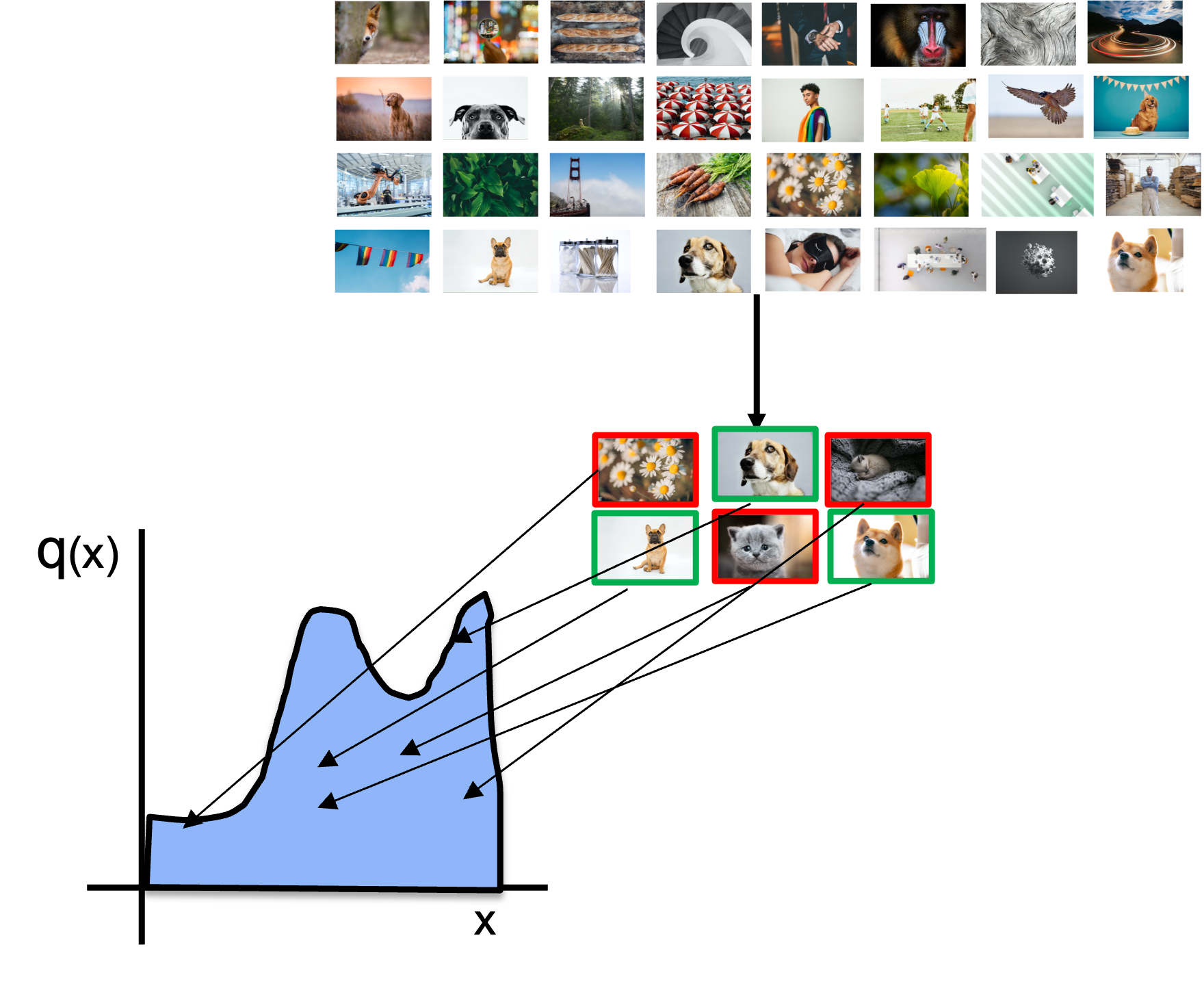
When trying to estimate F1, true positives, false negatives and false positives are the important pieces of information. Therefore, our sampling distribution prioritizes labeling these examples. Here, the distribution helps find far several true positives and false negatives in the form of dogs, but also some false positives in the form of cats that look like dogs:
Importance sampling has given us the theory to estimate the F-Score that would have been computed across the entire unlabeled dataset accurately, and with far lower variance than uniform random sampling. The efficiency of importance sampling depends on the shape of the importance distribution q. Prior work by Sawade et al. has worked out the theoretically optimal distribution q-star for F-Scores:
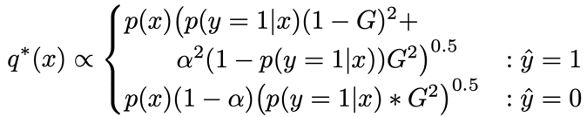
Where x is a given image in the domain, y is the ground-truth label, G is the ground-truth F-Score, and alpha is defined by the F-Score that we are estimating. While the details of this formulation are described in our paper, a key detail in Sawade’s method is that Sawade’s formulation of the sampling distribution q-star depends on knowing p(y=1|x), the probability that any given image is a ground-truth positive.
Sawade et al approximate this quantity by assuming the model is well-calibrated, but this assumption does not hold for many modern neural networks. This implies that we need to calibrate our models in order to leverage Sawade et al.’s work. But calibration in turn requires labeled datasets.
So now we’re in between a rock and a hard place:
- Importance sampling can reduce labeling budgets for validation
- Optimal importance sampling requires well-calibrated models
- Model calibration requires labeled data, which is the very thing we were trying to avoid.
We solve this cyclical dependence by introducing Active Calibration and Importance Sampling (ACIS), an algorithm that iteratively 1) labels samples according to our current estimate of the optimal importance sampling distribution,
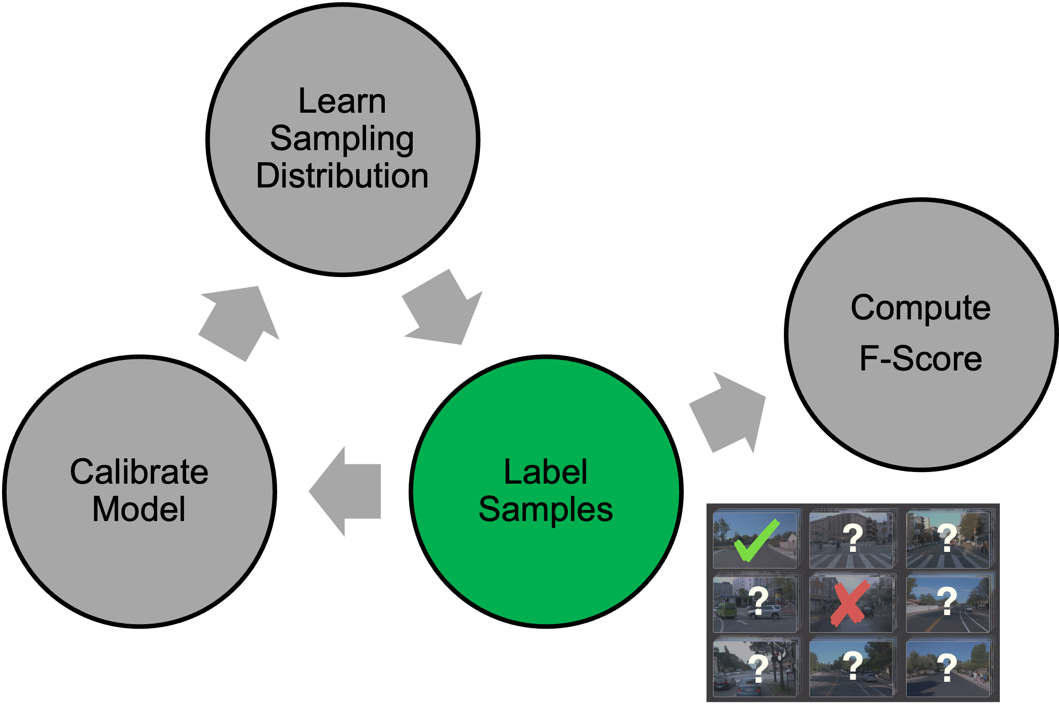
2) uses these samples both to calibrate model scores and to compute a current estimate of the F-Score,
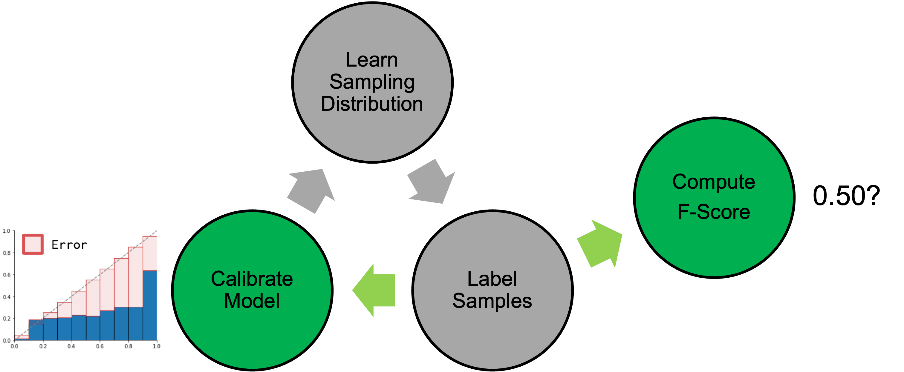
and 3) uses the calibrated model scores to compute a new estimate of the optimal sampling distribution for the next iteration.
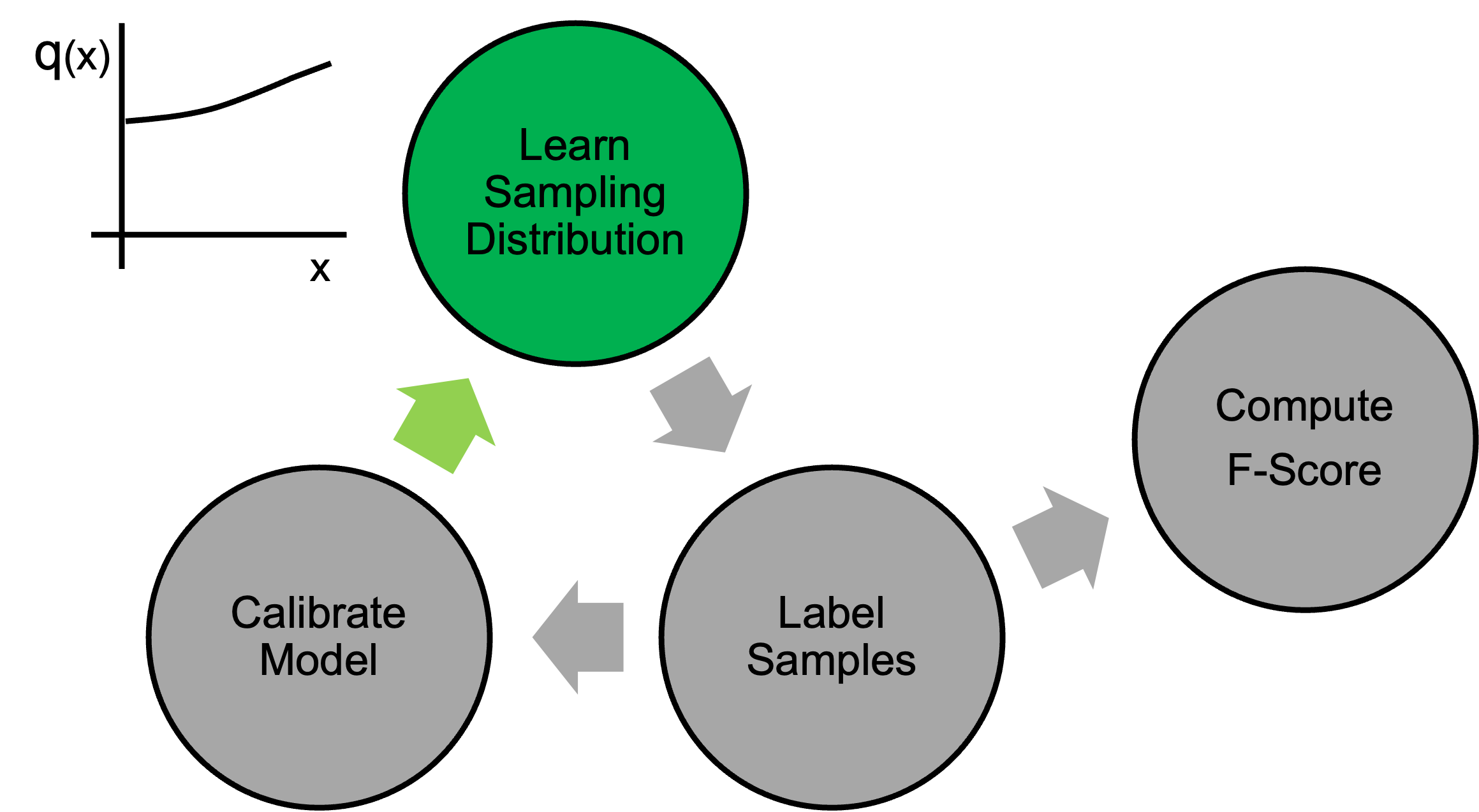
We repeat this process several times, labeling, calibrating, learning sampling distributions and generating estimates of the F-Score until our labeling budget has been met.
Improvements in variance performance
In order to test the impact of ACIS on validation performance, we validated binary classifiers on both the ImageNet and iNaturalist datasets. We train our classifiers on very small quantities of labeled data, using SwAV, SimCLRv2, and BYOL, well-known semi-supervised models with self-supervised pretraining. Note that since these models are trained on very little data, validation would become the primary labeling cost. We compared validation using ACIS against that of other popular baseline methods:
- Sawade et al.’s work (SAWADE), prior work on importance sampling which does not perform any model calibration.
- Isotonic regression (ISO), leveraging calibration without importance sampling in order to directly impute true positive, false positive, and false negative counts to estimate the F-Score
- Gaussian Mixture Models (GMM)
- Top-K sampling (TOP-K)
We measure performance in terms of the Mean Squared Error (MSE) of the estimated F1 compared to the F1 computed on the full dataset, and lower MSE values are better. We display experimetal results on log-log plots to highlight the dynamics between labeling budget and MSE:
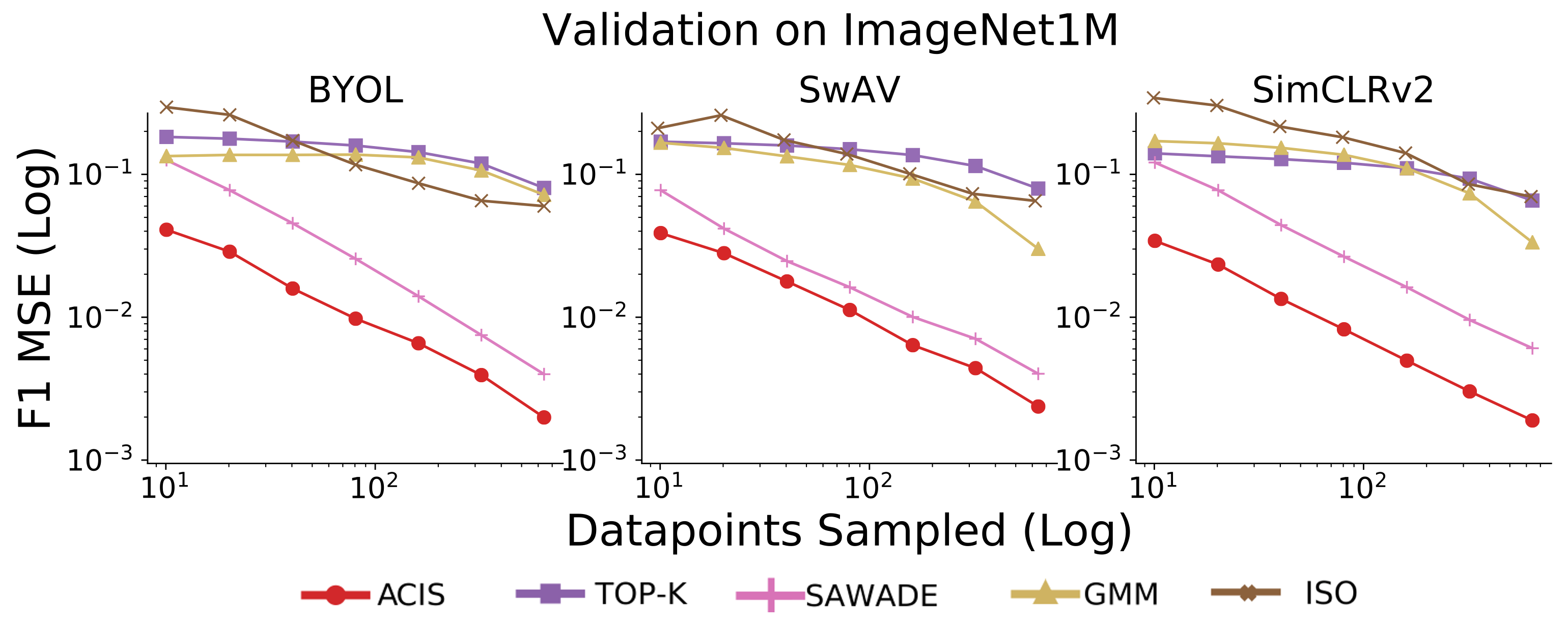
On ImageNet, ACIS outperforms both standalone importance sampling and standalone model calibration in terms of the MSE of estimated F1. We outperform the other baseline techniques as well. These trends hold across all three semi-supervised models, and across sampling regimes.
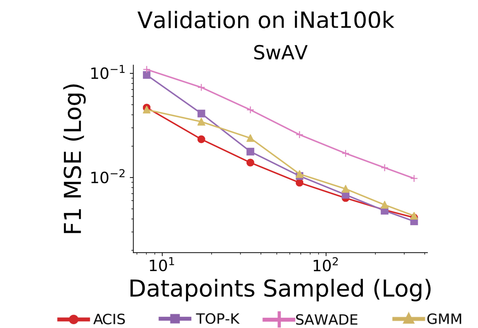
Overall the same trends apply for low sample budgets on iNaturalist—at fewer than 50 validation samples, ACIS outperforms the other methods. In this case the difference between ACIS and the other methods is low at the higher labeling counts. The reason for this is that some of the categories in iNaturalist are so rare that nearly all the true positives, false positives, and false negatives have been found by the time we have labeled 200 images.
Variance analysis
Keep in mind that ACIS is a statistical estimator, and it can have error. We have shown that this error is on average lower than baselines, but a practitioner looking to evaluate a model will only carry out the ACIS process once. That one estimate could have high error. Therefore, it is helpful to not only compute the ACIS estimate of the metric, but also the variance of that estimate.
We derive a theoretical estimator of ACIS’s variance, the details of which are in our paper:
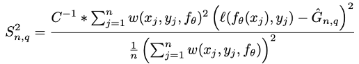
This is an estimate of the variance that is computed along with the F-score from the same labeled data, requiring no additional information.
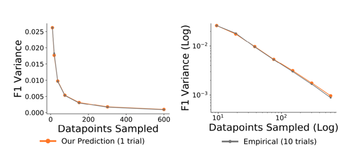
This estimator is empirically accurate across a range of dataset sizes, as the orange line showing the theoretical prediction closely matches the grey line showing the empirical variance from running 10 trials.
The theoretical derivation of the variance estimator is such that we can estimate the variance of any stochastically sampled validation set, including datasets sampled uniformly at random. If we view popular validation datasets such as ImageNet’s 50k validation set as a fixed-size randomized sample of the full data distribution, we can use our variance predictor to actually estimate the variance inherent in that validation dataset:
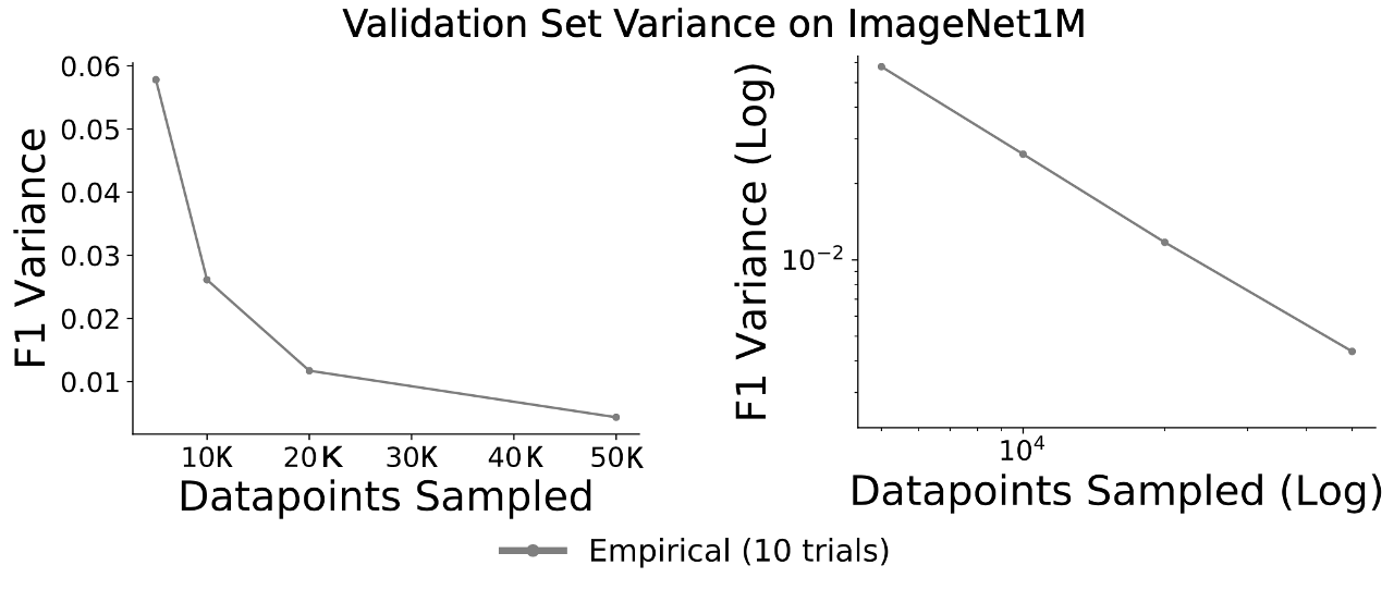
When validating binary classifiers using 50000 randomly selected images from the ImageNet dataset, we estimate that the average standard deviation in F1 estimates is 0.07. In other words, if we view the ImageNet validation set as a randomly selected sample from a much larger data distribution, the standard deviation of the typical category’s F1 is 0.07.
Reusing validation sets across models
Up until this point, we have discussed how to choose validation samples optimally for a given model. But a common validation task is to compare multiple models with the same validation set. So an interesting question is whether we can reuse validation sets across models. We have shown that ACIS is sample efficient at estimating F-scores, but when we reuse the model-specific datasets created for SimCLR and SwAV to validate BYOL, we achieve results that are not much worse in terms of MSE:
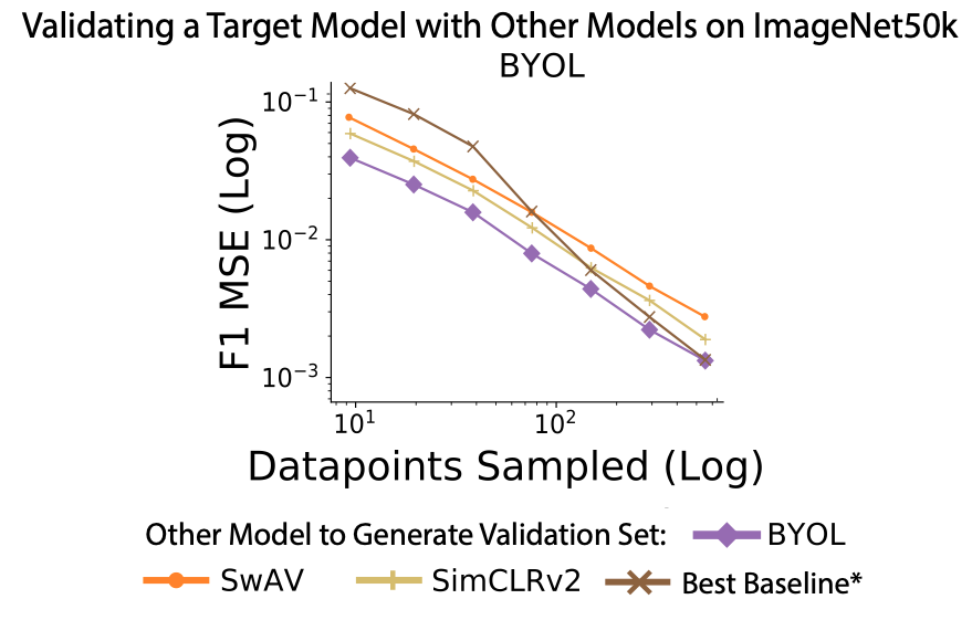
We often are actually competitive with model-specific baseline performance even when reusing the datasets originally curated for a different model.
Validation is stochastic
By framing model validation as a stochastic procedure, we have realized that active validation can substantially reduce labeling costs for model validation. Variance estimation makes ACIS practically usable in real-world settings, as does the empirical finding that ACIS-curated datasets can be reused effectively across model families.
We believe it is important to be mindful that all validation is a stochastic procedure. Even large datasets such as the ImageNet validation set are still finite-sized samples from a larger distribution. And for this reason we believe it is important to think about validation as a stochastic process and to be mindful of the potential variance in metrics we compute on those datasets.
Posts
-
Building Self-Improving LLM Agents: Paths Toward Lifelong Learning
Blog post authored jointly by Vishnu Sarukkai and Genghan Zhang
-
Diffusion Models and Policy Gradients Share a Common Structure
“True enough, this compass does not point north…It points to the thing you want most in this world.” – Jack Sparrow.
subscribe via RSS